A stable process can have "trends" within the range of its normal variation. Use the rules for randomization to ensure signs of an "unstable" system, giving support to the hypothesis that the changes resulted from your actions, before proceeding with the analysis of whether your improvement is "legitimate" (effective).
[Criteria for evidence of nonrandom influence (probability rules)]
A legitimate QIP is a process that achieves a benchmark rate of continuous improvement. The hypothesis is that any defect level, subjected to legitimate QIP, decreases at a constant rate, so that when plotted on semi-log paper against time, it falls on a straight line, making it easy to extrapolate.
- Plot the data and join the data points (trend line) to see if it looks like improvement is occurring
- Calculate the least square regression line, showing the resulting equation and R2 value for the data used
- Decide if the quality improvement program is consistently achieving improvement
- If so, classify the QIP as "legitimate", and proceed to calculate the half-life of improvement
Interpretation of R2
The value of R2 derived from the least square regression fit of the data is a measure of how well the QIP actions are correlated with the changes that occur. A value close to one indicates that there is a high statistical confidence level. A value close to zero implies that little in the observed data is explained by the model. How high R2 should be depends on the topic. In medical research, regression equations are often not accepted unless R2 is ≥ 0.99, while in behavioral or marketing studies where human behavior is involved, R2 values of about 0.15 or 0.2 are considered satisfactory. The average value in Schneiderman's paper was 0.77.
References:
-
Schneiderman A.M.
Setting quality goals.
American Society for Quality Control, 1988; April: 51-7. (PDF:72KB) www.schneiderman.com
Worked Example
|
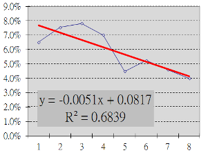
2012-Q1 6.50% 2012-Q2 7.54% 2012-Q3 7.81% 2012-Q4 7.01% 2013-Q1 4.48% 2013-Q2 5.25% 2013-Q3 4.60% 2013-Q4 3.99% |

|
One of the departments in our hospital is monitoring the number of accounts rejected by the insurance agency when applying for reimbursement. The results (rejection rate each quarter as a percentage of the total accounts) are shown for a two-year period of quality improvement activity.
The question we need to answer: is this a "legitimate" process, achieving reliable decrease in the rejection rate?
Initial inspection shows that despite an inital period where results seem to worsen, the overall trend appears to be downward. Using the steps on the left, the result is shown in the graph: the blue line connecting the data points is the trend line, the thick red straight line is the regression line derived from the least square method. The derived equation had a negative slope (-0.0051x) indicating a decreasing trend, and the R2 value (0.6839) confirms an acceptable correlation between actions and results.
The program meets the requirements for a "legitimate" QIP, and we can proceed to calculate the half-life of improvement and predict future results.
Since the time-between interval used in individual measurement control charts is an exponential distribution, the exponential regression equation eax+b is used. On the logarithmic scale axis, this becomes a straight line, and can be used for estimating imrprovement half-life as above.
i-type control chart
t-type control chart
g-type control chart