EWMA control chart|Tao Tips|

Similarly to the CUSUM chart, the EWMA chart is useful in detecting small shifts in the process mean. The performance of the EWMA control chart is approximately equivalent to that of the cuulative-sum control chart, and in some ways, it is easier to set up and operate. These charts are used to monitor th emean of a process based on samples taken from the process at given times (hours, shifts, days, weeks, months, etc). The measurements of the samples at a given time constitute a "subgroup". Each point is calculated where older points are weighted lower and lower. As with the CUSUM, the EWMA is typically used with individual observations (but can also be used for rational subgroups of size n > 1. Another option for single responses is I-chart. [I-chart]

The EWMA chart relies on the specification of a target value and a known or reliable estimate of the standard deviation. For this reason, it is best used after process control has been established to watch for early deviations from the target. Once a reliable estimate of the mean and standard deviation is available, the EWMA and CUSUM charts are useful in detecting smaller shifts in the process mean.

EWMA Calculations

The exponentially weighted moving average is defined as

[1] `z_i = lambda x_i + (1 - lambda) z_(i-1)`

where 0 ≤ λ ≤ 1 is a constant and the starting value (required with the first sample at i = 1) is the process target, so that `z_0 = mu_0`. Sometimes the average of preliminary data is used as the starting value of the EWMA, so that `z_0 = bar x`. The EWMA control chart is constructed by plotting z_i versus the sample number i (or time). The center line and control limits for are CL = μ₀, with control limits are

[2] `mu_0 ± L sigma sqrt((lambda / (2-lambda)) [1 - (1-lambda)^(2i)])`

Values of λ is specified by the user and is in the interval 0.05 ≤ λ ≤ 0.25 work well, with λ = 0.05, λ = 0.10, λ = 0.20 being popular choices. L = 3 (the usual 3-sigma limits) works reasonable well, although when λ is small, say λ ≤ 0.1, there is an advantage in reducing the width of the limits by using a value of L between 2.6 and 2.8. Using λ= 0.1 and L = 2.7 should result in an in-control ARL of ARL₀ ≅ 500 and for detecting a shift of one standard deviation in the process mean. For 0.2 and L=3 this will give an out of control signal after about 11 samples for a 1σ shift. The values of limits change with each successive subgroup, but ten to level off at around the tenth subgroup.

Rational subgroups

The target mean may be input directly, or it may be estimated from a series of subgroups. If it is estimated from the subgroups, the formula for the grand average is

[3] `bar (bar x) = (sum_(i=1)^k sum_(j=1)^(n_i) x_(ij)) / (sum_(i=1)^k n_i)`

When the sample size is variable across subgroups, a weighted approach is recommended for estimating sigma.

[4] `hat sigma = bar s = [(sum_(i=1)^k ((n_i - 1) s_i^2)) / ((sum_(i=1)^k n_i) - k) ]^(1/2)`

If rational subgroups of size n > 1 are used, then simply replace `x_i` with `bar x_i` and `sigma` with `sigma_(bar x) = sigma / sqrt(n)` in the equations.

EWMA example (n=1)

Data

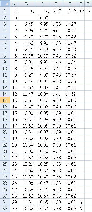
The target value for the process mean is 10.0 with a σ = 1.


                 9.45  7.99  9.29 11.66 12.16 10.18  8.04 11.46  9.20 10.34 

                 9.03 11.47 10.51  9.40 10.08  9.37 10.62 10.31  8.52 10.84 
 
                10.90  9.33 12.29 11.50 10.60 11.08 10.38 11.62 11.31 10.52

{Montgomery p.335}

Steps to complete Figure 1

1. Type the column headings into your Excel sheet. Type the text in quotation marks, but without the quotation marks.

A1 : "i " (number of the sample subgroup)
B1 : "x_i " (the data from above for each sample)
C1 : "z_i " (EWMA value calculated for each sample)
D1 : "LCL " (lower control limit)
E1 : "UCL " (upper control limit)
F1 : "Y+ " (Y = yes if EWMA value exceeds UCL)
G1 : "Y- " (Y = yes if EWMA value is below LCL)

2. Complete column A.

A2 : "0"
A3 : "=A2+1"
drag (copy formula) A3 to A32 so that …
A32 : "=A30+1"
check that the result is a sample sequence from A2:A32 of 0~30

3. Type the data from your project (see above [Data]) into the range B3:B32.

4. Choose an area of the Excel sheet below your data for process parameters, for example, starting at A34.

  A34 : "`bar x`", B34 : "10.00"
  A35 : "`sigma`", B35 : "1.0"
  A36 : "`lambda`", B36 : "0.1"
  A37 : "L", B37 : "2.7"

Figure 1. Aggregate data

5. Choose an area of the Excel sheet below your data for process parameters, for example, starting at A34.

C2 : "=$B$34"

6. Calculate the rest of the EWMA column

C3: "=B3*$B$36+(1-$B$36)*C2"
Select C3, then drag (copy formula) through to C32 so that …
C32: "=B32*$B$36+(1-$B$36)*C31"

7. Set up columns for control limits, to facilitate drawing the lines on the graph later.

D3: "=$B$34+$B$37*$B$35*SQRT(($B$36/(2-$B$36))*(1-POWER((1-$B$36),(2*A3))))"
E3: "=$B$34-$B$37*$B$35*SQRT(($B$36/(2-$B$36))*(1-POWER((1-$B$36),(2*A3))))"
Select D3 together with E3, then drag (copy formula) through to E32 so that …
D32: "=$B$34+$B$37*$B$35*SQRT(($B$36/(2-$B$36))*(1-POWER((1-$B$36),(2*A32))))"
E32: "=$B$34-$B$37*$B$35*SQRT(($B$36/(2-$B$36))*(1-POWER((1-$B$36),(2*A32))))"
Check that your results agree with LCL and UCL in Table 1.

Notice that the control limits increase in width as i increases from i = 1, 2, …, until they stabilize at the steady-state values of LCL = 9.38 and UCL = 10.62.

8. Test for whether control limits are exceeded. If the `EWMA_i` exceeds `UCL_i` or `EWMA_i` is below `LCL_i`, then flag the sample with the letter "Y" (=Yes)

F3: "=IF(C3>E3,"Y","")"
G3: "=IF(C3<=D3,"Y","")"
Select F3 together with G3, then drag (copy formula) through to G32 so that …
F32: "=IF(C32>E32,"Y","")"
G32: "=IF(C32<=D32,"Y","")"
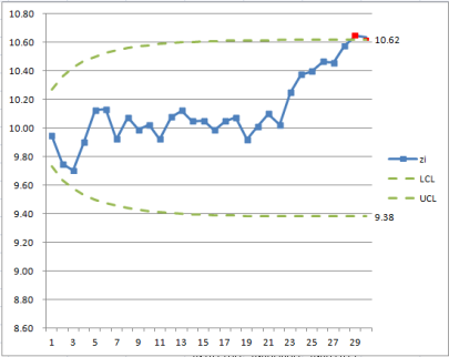
Check that your result is a "Y" in cell F31 and F32.

The EWMA control chart (Figure 1) signals that the process is out of control at observation 29.

Table 1. EWMA data (n=1) table.

Figure 2. EWMA graph of data (n=1) in Table 1.

Rational subgroup (n>1)

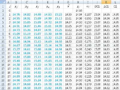
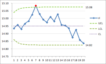
To monitor a process for a change in the mean, subgroup samples of five observations were made each day. Each line in the data below represents the five observations for one day. The monitoring starts at the first line, and was continued for 20 days (the bottom line of data). (User-defined parameters to use in calculations are λ = 0.3 and L = 1.5).

Data


                   14.76  14.82  14.88  14.83  15.23

                   14.95  14.91  15.09  14.99  15.13

                   14.50  15.05  15.09  14.72  14.97

                   14.91  14.87  15.46  15.01  14.99

                   14.73  15.36  14.87  14.91  15.25

                   15.09  15.19  15.07  15.30  14.98

                   15.34  15.39  14.82  15.32  15.23

                   14.80  14.94  15.15  14.69  14.93

                   14.67  15.08  14.88  15.14  14.78

                   15.27  14.61  15.00  14.84  14.94

                   15.34  14.84  15.32  14.81  15.17

                   14.84  15.00  15.13  14.68  14.91

                   15.40  15.03  15.05  15.03  15.18

                   14.50  14.77  15.22  14.70  14.80

                   14.81  15.01  14.65  15.13  15.12

                   14.82  15.01  14.82  14.83  15.00

                   14.89  14.90  14.60  14.40  14.88

                   14.90  15.29  15.14  15.20  14.70

                   14.77  14.60  14.45  14.78  14.91

                   14.80  14.58  14.69  15.02  14.85

SAS User's Guide

1. Type the column headings into your Excel sheet. Type the text in quotation marks, but without the quotation marks.

A1 : "i " (number of the sample subgroup)
B1 : "x₁ " (first of five observations from the daily sample)
C1 : "x₂ " (second of five observations from the daily sample)
D1 : "x₃ " (third of five observations from the daily sample)
E1 : "x₄ " (fourth of five observations from the daily sample)
F1 : "x₅ " (fifth of five observations from the daily sample)
G1 : "`bar x`" (average of daily sample)
H1 : "z_i " (EWMA value for daily sample)
I1 : "σ_i " (standard deviation for daily sample)
J1 : "UCL " (standard deviation for daily sample)
K1 : "UCL " (lower control limit)
L1 : "CL " (center line)

2. Set up sequence number for subgroups in column A.

A1 : "i "
A2 : "0"
A3 : "=A2+1"
drag (copy formula) A3 to A22 so that …
A22 : "=A21+1"
check that the result is a sample sequence from A2:A22 of 0~20

3. Enter data in columns B..F for i = 1 to 20.

4. Calculate subgroup mean in Column G3.

G3 : "=AVERAGE(B3:F3)"
drag (copy formula) G3 to G22 so that …
G22 : "=AVERAGE(B22:F22)"
check that the result the same as in Table 2.

5. Calculate subgroup standard deviation in column I.

I3: "=STDEV(B3:F3)"
drag (copy formula) I3 to I22 so that …
I22 : "=STDEV(B22:F22)"
check that the result the same as in Table 2.

6. Set the starting point for EWMA calculations to the process mean

H2: "=$H$25"

7. Choose an area of the Excel sheet below your data for process parameters, for example, starting at G25.

Figure 3. Parameters (n>1)

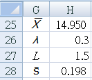
  G25 : "`bar bar x`" weighted mean of subgroup means
  G26 : "`lambda`" user-defined
  G27 : "L" user-defined
  G28 : "`bar bar S`" average of subgroup standard deviations

H25 : "=AVERAGE($B$3:$F$22)"
H28 : "=AVERAGE($I$3:$I$22)"

8. Calculate EWMA for each subgroup in column H

H3: "=$H$26*G3+(1-$H$26)*H2"
drag (copy formula) H3 to H22 so that …
H22 : "=$H$26*G3+(1-$H$26)*H21"
check that the result the same as in Table 2.

9. Calculate UCL i=1 into J3.

J3: "=$H$2+$H$27*$H$28*SQRT(($H$26/(2-$H$26))*(1-POWER((1-$H$26),(2*A3))))"

10. Calculate LCL i=1 into K3.

K3: "=$H$2-$H$27*$H$28*SQRT(($H$26/(2-$H$26))*(1-POWER((1-$H$26),(2*A3))))"
Select J3 together with K3, then drag (copy formula) to K22 so that …
K22 : "=$H$2-$H$27*$H$28*SQRT(($H$26/(2-$H$26))*(1-POWER((1-$H$26),(2*A22))))"
check that the result the same as in Table 2.

11. Add another column L for "CL" on the graph, set the entire column equal to the process mean

L3: "=$H$25"
drag (copy formula) L3 to L22

12. Draw your EWMA graph. Note that `EWMA_(i=7)` lies above the UCL, indicating an out-of-control process.

Table 2. EWMA data (n>1) table.

Figure 4. EWMA graph of data (n>1) in Table 2.

Variable sample size

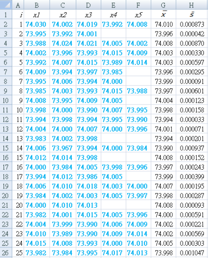
Table 3. EWMA calculations for variable samples (n>1).

Montgomery p.218

For unequal size sample subgroups, use the same Excel equation to calculate the weighted mean of subgroup averages.

H25: "=AVERAGE($B$2:$F$26)"
`bar bar x` = 74.001

But for the weighted average of standard deviations (H28), the equation

`hat sigma = bar s = [(sum_(i=1)^k ((n_i - 1) s_i^2)) / ((sum_(i=1)^k n_i) - k) ]^(1/2)`

can be calculated by changing the Excel formula for standard deviation in column H to:

H3 : "=(COUNT(B2:F2)-1)*POWER(STDEV(B2:F2),2)"
Select cell H3 and drag (copy formula) through to H26.

After which, for the weighted average of standard deviations `bar S`, change the Excel formula in H28 to:

H28 : "=POWER(SUM($H$2:$H$26)/(COUNT($B$2:$F$26)-COUNT($H$2:$H$26)),0.5)"
`bar S` = 0.01029

The Excel formulas for UCL and LCL do not need to be modified. Their values will show the effects of these modifications.