Likert-item Surveys Treated As Normal Distribution
Subjective assessment of something that cannot be measured objectively (such as patient satisfaction) is "ordered categorical" data type. For example, a patient may classify their degree of { satisfaction as: Unsatisfied / poorly satisfied / neutral / somewhat satisfied / satisfied } or their degree of pain as { minimal / moderate /severe /unbearable }. Data of this type are also called [ordinal] data.
With ordinal data, we cannot say that "somewhat satisfied" is twice as good as "poorly satisfied", or that the difference between each of the levels (for example, the change from "unsatisfied" ⇒ "poorly satisfied" compared to the change from "somewhat satisfied" ⇒ "satisfied") is equivalent. When ordered categories are numbered, as with the Likert scale for satisfaction surveys, the temptation to treat these numbers as statistically meaningful must be resisted. For example, it is not sensible to calculate the AVERAGE (mean) level of satisfaction. The only information the numbers contain is in the ordering. Parametric methods are based on calculating means and standard deviations, so they are inappropriate for ordered categorical data such as satisfaction surveys. (Altman [1] p.180)
That having been said, using Google to search returns many examles of average and standard deviations being calculated for satisfaction surveys (for example, Press-Ganey surveys in the US). And since our hospitals report to the Taiwan Society of Hospital Executives which uses the average of a five-point Likert scale as the satisfaction indicator, our web pages provide these calculations as follows.
Example
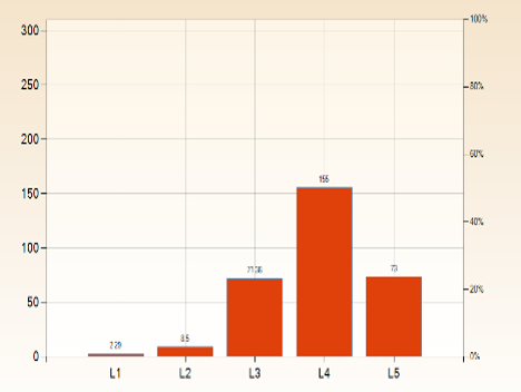
In response to a question in a survey, where respondents could choose from a Likert scale of 1 to 5, the results for that item were:
{4, 5, 4, 5, 5, 5, 5, 3, 4, 3}
| Statistic | Excel function | Result |
|---|---|---|
| Mean | = AVERAGE(4, 5, 4, 5, 5, 5, 5, 3, 4, 3) | = 4.3 |
| Standard Deviation | = STDEV(4, 5, 4, 5, 5, 5, 5, 3, 4, 3) | = 0.823273 |
| Count | = COUNT(4, 5, 4, 5, 5, 5, 5, 3, 4, 3) | = 10 |
| Confidence Interval | = CONFIDENCE(0.05, STDEV(), COUNT()) | |
| = CONFIDENCE(0.05, 0.823273, 10) | = 0.51027 |
However, since our web pages show grouped survey data, this section shows you how the same results are obtained using grouped data.
- The class interval c is a constant which is equidistant (=1) for the Likert scale used in our satisfaction surveys
- u is the Likert value (one of 1 to 5)
- f is the frequency that the Likert value was selected by people answering the survey
- s is the SAMPLE standard deviation.
| Grouped Data from Survey | Calculations | |||||||||
|---|---|---|---|---|---|---|---|---|---|---|
| A | B | C | D | E | F | G | H | I | J | K |
| 1 | Likert Score | u | 1 | 2 | 3 | 4 | 5 | Σ | ||
| 2 | Vote frequency | f | 0 | 0 | 2 | 3 | 5 | =SUM(D2:H2) | 10 | =Σf |
| 3 | Grouped data | fu 2 | 0 | 0 | 18 | 48 | 125 | =SUM(D3:H3) | 191 | =Σfu 2 |
| 4 | Grouped data | fu | 0 | 0 | 6 | 12 | 25 | =SUM(D4:H4) | 43 | =Σfu |
`= 0.823273`
which is the same result as Table 1 which used the raw data ⇒ STDEV(4, 5, 4, 5, 5, 5, 5, 3, 4, 3)
`= 0.823273`
which is the same result as Table 1 which used the raw data ⇒ AVERAGE(4, 5, 4, 5, 5, 5, 5, 3, 4, 3)
which is the same result as Table 1 which used the raw data ⇒ CONFIDENCE(0.5, 0.823273, 10)
`= 4.3 ` `(3.78973 ∼ 4.81027)`
Or as a percentage of the maximum Likert score of 5
Confidence Intervals
A confidence interval is a range of values that is used to describe the uncertainty around a point estimate of a quantity such as a satisfaction rate and are a measure of the variability in the data. Confidence intervals are calculated with a stated probability (for example 95%), and we say that there is a 95% chance that the confidence interval covers the true value. Most confidence intervals are calculated as 95% confidence intervals for the same reason that most statistical tests are done at the 0.05 level ‐ in other words, only because it's conventional. It is completely arbitrary that we consider a result that would happen only 5 out of 100 times by chance as being statistically significant, while we consider one happening 6 out of 100 times as not being statistically significant. Confidence intervals do not account for several other sources of uncertainty in point estimates, including missing or incomplete data or other data errors, or bias resulting from non-response or poor data collection.
Normal Distribution
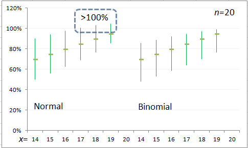
The Normal approximation is reasonable when both np and n(1-p) exceed 5, hence is only valid for large samples ( > 30); however, the response rate in employee satisfaction surveys, or in stratification of any satisfaction survey, often falls below these levels. In this case, it is recommended to accumulate data longer-term (e.g. six months or one year). For example, if `hat p` = 0.1, then N should be at least 50 and if `hat p` = 0.01, then N should be at least 500. Criteria for choosing a sample size in order to guarantee detecting a change are discussed elsewhere, nd are important when designing control charts.
在此公式中,`hat p` 是由統計樣本估計出來的比例,n 是樣本數,z(1-α/2) 是標準常態分布的 (1-α/2) 百分位數(以 95% 信賴區間來說,這個值為 1.96 。當 np及 n(1-p) 都大於 5 的時候,用常態近似法是合理的,因此,他只適用於大樣本的資料 (≥ 30); 然而,像員工滿意度調查的回收率或任何調查的分層分析,其樣本數往往會在這個標準之下 (n < 30)。In many simple situations, especially those involving normally-distributed data, or large samples of data from other distributions, the normal approximation may be used to calculate the confidence interval. In this method, confidence intervals are given by:
where `hat p` is the proportion estimated from the statistical sample, `n` is the sample size, and ` z_(1 - \alpha \/2) ` is the 1-α/2 percentile of a standard normal distribution (for 95% CI, this value is 1.96).
Excellence
(top-two-box) indicator: a total of 86 people answered the survey, of whom 33 gave a score of 4 out of a maximum of 5, and 12 gave the maximum 5.
Therefore the numerator for "excellence" (top-two-box) indictor was 33 + 12 = 45, and the denominator was 86.
p = 45 ÷ 86 = 0.523
1-p = 0.477
n = 86
Normal approximation requires both np and n(1-p) exceed 5, hence:
np = 86 x 0.523 = 44.978
n(1-p) = 86 x (1-0.523) = 41.02
indeed both are the same > 5。
Using the above equation,
95% CI
`
= 0.523 ± 1.96 sqrt((0.523 × 0.477) / 86)
`
`
= 0.523 ± 0.105
`
Excellence (top-box) index = 52.3% (LCL: 41.8%, UCL: 62.9%) or when explaining the result to others, ought to say it ranges between 41.8% and 62.9%.
The two percentages on the far right of each line of our web pages reporting satisfaction survey results are the upper and lower 95% confidence intervals for the indicator immediately to their left.
Binomial Distribution
In the past, many analysts recommended computing "exact" confidence intervals directly from the binomial distribution when the sample size is small. However, exact confidence intervals tend to be conservative (too wide). Agresti & Coull [6] showed that the score interval works better in almost all circumstances than exact intervals, even for the smallest sample sizes. Therefore, the score interval is recommended for all sample sizes and is the method used on this website for satisfaction surveys.
The score interval for calculating confidence intervals for binomial proportions is found by solving the quadratic equation:

where n is the sample size, x is the number of successes, zα/2 is the α/2-level normal deviate (e.g. 1.96 for 95% intervals), and ` hat p` is the confidence limit to be estimated.
With this method, the lower limit cannot be negative, which is not true for the Normal approximation of the Binomial distribution.
Confidence intervals for the binomial distribution are not symmetric about the observed proportion unless p ≅ 0.5.
"Excellence" (top-two-box) indicator: a total of 20 people answered the survey, of whom 3 gave a score of 4 out of a maximum of 5, and 1 gave the maximum 5.
Therefore, the numerator x for the top-two-box indicator was 3 + 1 = 4, and the numerator n was 20. ` hat p ` = x ÷ n = 4 ÷ 20 = 0.2 (20%)
Using the above equation: 95% CI
Using the above equation, the top-two-box indicator = 20% (UCL: 8.1%, UCL: 41.6%), or when reporting, should say it was in the range 8.1% ~ 41.6%. Note that the result is asymmetric around the mean, the distance from the mean being 11.9% for the lower limit and 21.6% for the upper limit.


Calculate using Excel
95% CI (change to other values if required)
Number of surveys (denominator)
Number of surveys given desired response, for example, top-two-box (numerator)
LCL : 0.080656353
References
- Altman DG. Practical statistics for medical research. Chapman & Hall/CRC, 1991. pp.231-2
- Spiegel MR. Shaum's outline of theory and problems of statistics. McGraw-Hill Inc. 1972. p.78-9 section 4.16
- Pezzullo JC. Online calculator for Exact Binomial and Poisson Confidence Intervals statpages.org/confint.html
- Bhaskar. Online calculator for Mean & Standard Deviation from frequency table & grouped data: knowpapa.com/sd-freq/
- Vollset SE. Confidence intervals for a binomial proportion. Statistics in Medicine 1993; 12(9): 809-823.
- Agresti A & Coull BA. Approximate is better than "exact" for interval estimation of binomial proportions, The American Statistician, 1998; 52(2): 119-126.